
The Causal Revolution as the Summit of Scientific-Technological-Industrial Revolutions
July 11, 2021


Background
This post aims to provide further insight to readers of “Book of Why” (BOW) (Pearl and Mackenzie, 2018) on Lord’s paradox and the simple way this decades-old paradox was resolved when cast in causal language. To recap, Lord’s paradox (Lord, 1967; Pearl, 2016) involves two statisticians, each using what seems to be a reasonable strategy of analysis, yet reaching opposite conclusions when examining the data shown in Fig. 1 (a) below.
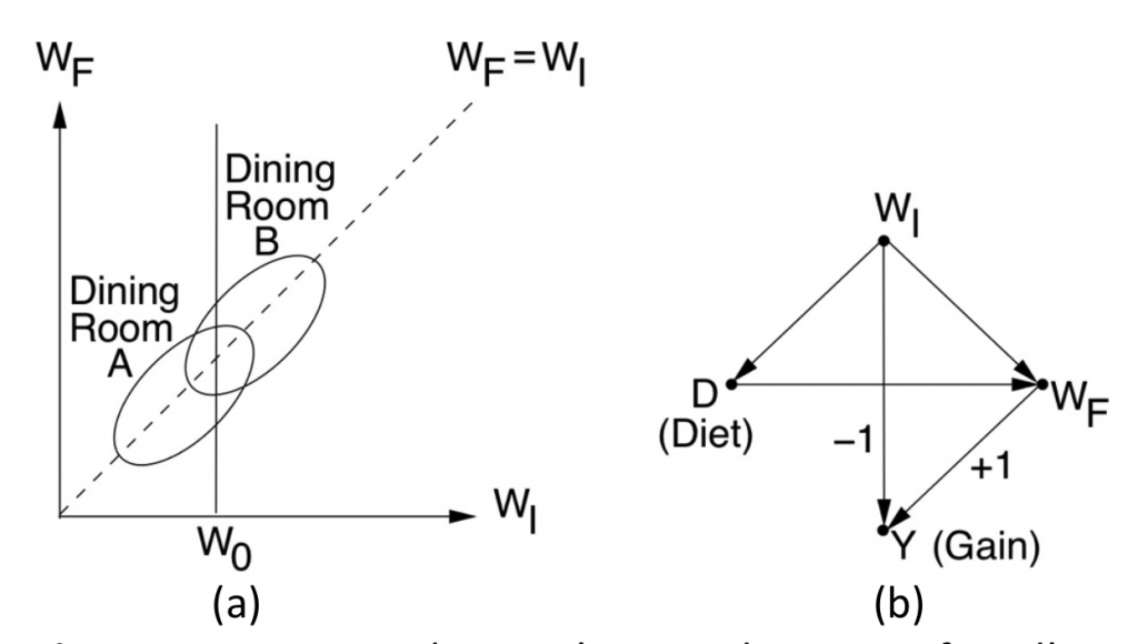
Figure 1: Wainer and Brown’s revised version of Lord’s paradox and the corresponding causal diagram.
The story, in the form described by Wainer and Brown (2017) reads:
“A large university is interested in investigating the effects on the students of the diet provided in the university dining halls …. Various types of data are gathered. In particular, the weight of each student at the time of his arrival in September and his weight the following June (WF) are recorded.”
The first statistician (named John) looks at the weight gains associated with the two dining halls, find them equally distributed, and naturally concludes that Diet has no effect on Gain. The second statistician (named Jane) uses the initial weight (WI) as a covariate and finds that, for every level of WI, the final weight (WF) distribution for Hall B is shifted above that of Hall A. Thus concluding Diet has an effect on Gain. Who is right?
The Book of Why resolved this paradox using causal analysis. First, noting that at issue is “the effect of Diet on weight Gain”, a causal model is postulated, in the form of the diagram of Fig. 1(b). Second, noting the WIis the only confounder of Diet and Gain, Jane was declared “unambiguously correct” and John “incorrect”.
The Critics
The simplicity of this solution invariably evokes skepticism among statisticians. “But how can we be sure of the diagram?” they ask. This kind of skepticism is natural since, statisticians are not trained in postulating causal assumptions, that is, assumptions that cannot be articulated in the language of mainstream statistics, and cannot therefore be tested using the available data. However, after reminding the critics that the contention between John and Jane surrounds the notion of “effect”, and that “effect” is a causal, not statistical notion, enlightened statisticians accept the idea that diagrams need to be drawn and that the one in Fig. 1(b) is reasonable; its main assumptions are: Diet does not affect the initial weight and the initial weight is the only factor affecting both Diet and final weight.
A series of recent posts by S. Senn, however, introduced a new line of criticism into our story (Senn, 2019). It focuses on the process by which the data of Fig. 1(a) was generated, and invokes RCT considerations such as block design, experiments with many halls, analysis of variance, standard errors, and more. Statisticians among my Twitter followers “liked” Senn’s critiques and I am not sure whether they were convinced by my argument that Lord’s paradox has nothing to do with experimental procedures. In other words, the conflict between John and Jane persists even when the data is generated by clean and un-complicated process, as the one depicted in Fig. 1(b).
Senn’s critiques can be summarized thus (quoted):
“I applied John Nedler’s experimental calculus [5, 6] … and came to the conclusion that the second statistician’s solution is only correct given an untestable assumption and that even if the assumption were correct and hence the estimate were appropriate, the estimated standard error would almost certainly be wrong.”
My response was:
Lord’s paradox is about causal effects of Diet. In your words: “diet has no effect” according to John and “diet does have an effect” according to Jane. We know that, inevitably, every analysis of “effects” must rely on causal, hence “untestable assumptions”. So BOW did a superb job in calling the attention of analysts to the fact that the nature of Lord’s paradox is causal, hence outside the province of mainstream statistical analysis. This explains why I agree with your conclusion that “the second statistician’s solution is only correct given an untestable assumption”. Had you concluded that we can decide who is correct without relying on “an untestable assumption”, you and Nelder would have been the first mortals to demonstrate the impossible, namely, that assumption-free correlation does imply causation.
Now let me explain why your last conclusion also attests to the success of BOW. You conclude: “even if the assumption were correct, … the estimated standard error would almost certainly be wrong.”
The beauty of Lord’s paradox is that it demonstrates the surprising clash between John and Jane in purely qualitative terms, with no appeal to numbers, standard errors, or confidence intervals. Luckily, the surprising clash persists in the asymptotic limit where Lord’s ellipses represent infinite samples, tightly packed into those two elliptical clouds.
Some people consider this asymptotic abstraction to be a “limitation” of graphical models. I consider it a blessing and a virtue, enabling us, again, to separate things that matter (clash over causal effects) from those that don’t (sample variability, standard errors, p-values etc.). More generally, it permits us to separate issues of estimation, that is, going from samples to distributions, from those of identification, that is, going from distributions to cause-effect relationships. BOW goes to great length explaining why this last stage presented an insurmountable hurdle to analysts lacking the appropriate language of causation.
Note that BOW declares Jane to be “unambiguously correct” in the context of the causal assumptions displayed in the diagram (Fig.1 (b)) where Diet is shown NOT to influence initial weight, and the initial weight is shown to be the (only) factor that makes students prefer one diet or another. Changing these assumptions may lead to another problem and another resolution but, once we agree with the assumptions our choice of Jane as the correct statistician is “unambiguously correct”
As an example (requested on Twitter) if dining halls have their own effect on weight gain (say Hall-A provides free weight-watching instructions to diners) our model will change as depicted in Fig 2. In this setup, WI is no longer a sole confounder and both WI and Hall need to be adjusted to obtain the effect of Diet on Gain. In other words, Jane will no longer be “correct” unless she analyzes each stratum of the Diet-Hall combination and finds preference of Diet-A over Diet-B.
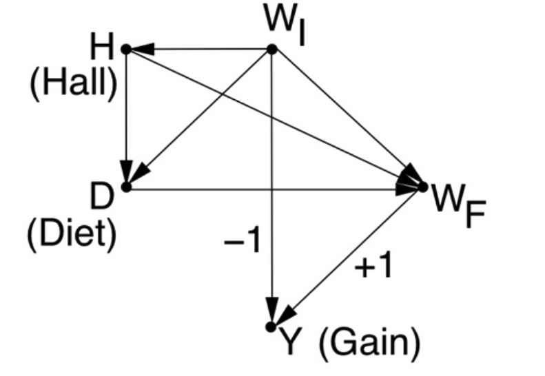
Figure 2: Separating Diet from Hall in Lord’s Story
New Insights
The upsurge of interest in Lord’s paradox gives me an opportunity to elaborate on another interesting aspect of our Diet-weight model, Fig. 1.
Having concluded that Statistician-2 (Jane) is “unambiguously correct” and that Statistician-1 (John) is wrong, an astute reader would ask: “And what about the sure-thing principle? Isn’t the overall gain just an average of the stratum-specific gains?” (where each stratum represents a level of the initial weight WI). Previously, in the original version of the paradox (Fig. 6.8 of BOW) we dismissed this intuition by noting that WI was affected by the causal variable (Sex) but, now, with the arrow pointing from WI to D we can no longer use this argument. Indeed, the diagram tells us (using the back-door criterion) that the causal effect of D on Y can be obtained by adjusting for the (only) confounder, WI, yielding:
P(Y|do(Diet)) = ∑WIP(Y|Diet,WI) P(WI)
In other words, the overall gain resulting from administering a given diet to everyone is none other but the gain observed in a given diet-weight group, averaged over the weight. How is it possible then for the latter to be positive (as seen from the shifted ellipses) and, simultaneously, for the former to be zero (as seen by the perfect alignment of the ellipses along the WI = WF line)
One would be tempted to suggest that data matching the ellipses of Fig 6.9(a) can never be generated by the model of Fig. 6.9(b) , in which WIis the only confounder? But this could not possibly be the case, because we know that the model has no refuting implications, so it cannot be refuted by the position of the two ellipses.
The answer is that the sure-thing principle applies to causal effects, not to statistical associations. The perfect alignment of the ellipses does not mean that the effect of Diet on Gain is zero; it means only that the Gain is statistically independent of Diet:
P(Gain|Diet=A) = P(Gain|Diet=B)
not that Gain is causally unaffected by Diet. In other words, the equality above does not imply the equality
P(Gain|do(Diet=A)) = P(Gain|do(Diet=B))
which statistician-1 (John) wants us to believe.
Our astute student will of course question this explanation and, pointing to Fig. 1(b), will ask: How can Gain be independent of Diet when the diagram shows them connected? The answer is that the three paths connecting Diet and Gain cancel each other in such a way that an overall independence shows up in the data,
Conclusions
Lord’s paradox starts with a clash between two strong intuitions: (1) To get the effect we want, we must make “proper allowances” for uncontrolled preexisting differences between groups” (i.e. initial weights) and (2) The overall effect (of Diet on Gain) is just the average of the stratum-specific effects. Like the bulk of human intuitions, these two are CAUSAL. Therefore, to reconcile the apparent clash between them we need a causal language; statistics alone won’t do.
The difficulties that generations of statisticians have had in resolving this apparent clash stem from lacking a formal language to express the two intuitions as well as the conditions under which they are applicable. Missing were: (1) A calculus of “effects” and its associated causal sure-thing principle and (2) a criterion (back door) for deciding when “proper allowances for preexisting conditions” is warranted. We are now in possession of these two ingredients, and we should enjoy the power of causal analysis to resolve this paradox, which generations of statisticians have found intriguing, if not vexing. We should also feel empowered to resolve all the paradoxes that surface from the causation-association confusion that our textbooks have bestowed upon us.
References
Lord, F.M. “A paradox in the interpretation of group comparisons,” Psychological Bulletin, 68(5):304-305, 1967.
Pearl, J. “Lord’s Paradox Revisited — (Oh Lord! Kumbaya!)”, Journal of Causal Inference, Causal, Casual, and Curious Section, 4(2), September 2016. https://ftp.cs.ucla.edu/pub/stat_ser/r436.pdf
Pearl, J. and Mackenzie, D. Book of Why, NY: Basic Books, 2018. http://bayes.cs.ucla.edu/WHY/
Senn, S. “Red herrings and the art of cause fishing: Lord’s Paradox revisited” (Guest post) August 2, 2019. https://errorstatistics.com/2019/08/02/s-senn-red-herrings-and-the-art-of-cause-fishing-lords-paradox-revisited-guest-post/
Wainer and Brown, L.M., “Three statistical paradoxes in the interpretation of group differences: Illustrated with medical school admission and licensing data,” in C.R. Rao and S. Sinharay (Eds.), Handbook of Statistics 26: Psychometrics, North Holland: Elsevier B.V., pp. 893-918, 2007.
The Causal Revolution as the Summit of Scientific-Technological-Industrial Revolutions
July 11, 2021

April 1, 2021

Why machine learning struggles with causality
March 28, 2021

The Domestication of Causal Reasoning
December 28, 2020
AI World Society - Powered by BGF