Causal Inference 360

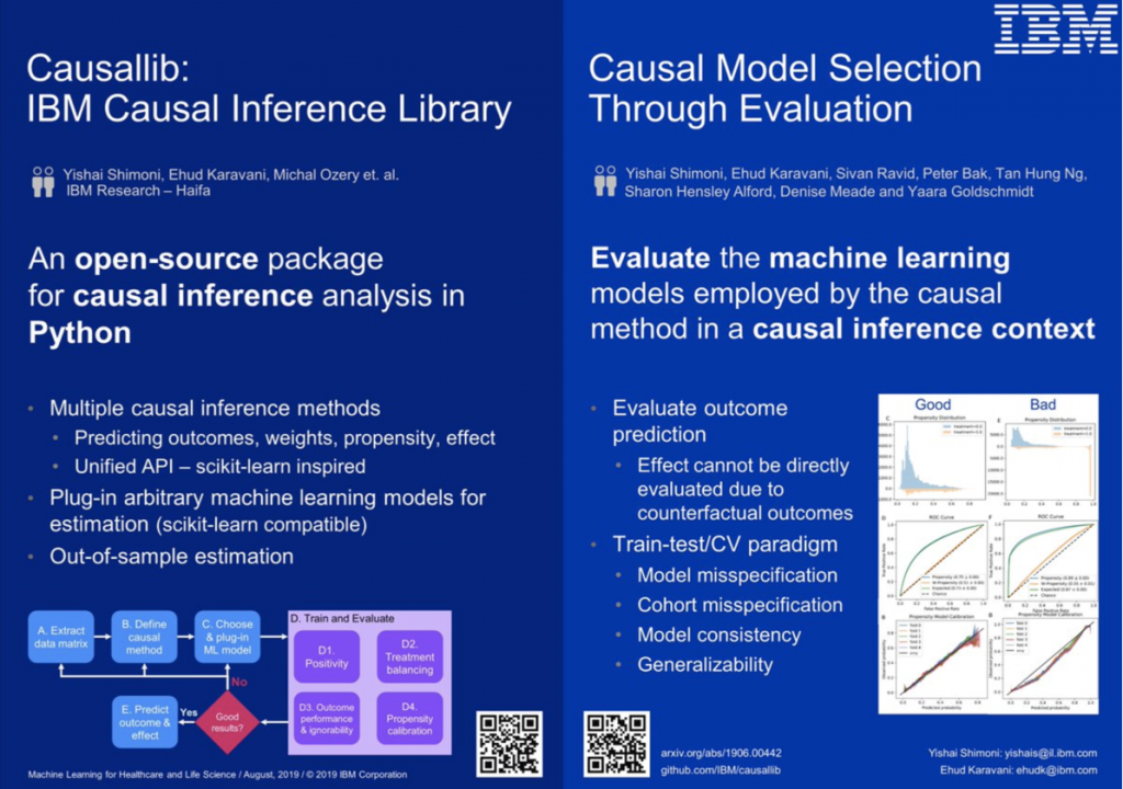
A Python package for inferring causal effects from observational data.

Description

Causal inference analysis enables estimating the causal effect of an intervention on some outcome from real-world non-experimental observational data.

This package provides a suite of causal methods, under a unified scikit-learn-inspired API.
It implements meta-algorithms that allow plugging in arbitrarily complex machine learning models. This modular approach supports highly-flexible causal modelling.
The fit-and-predict-like API makes it possible to train on one set of examples and estimate an effect on the other (out-of-bag), which allows for a more “honest”¹ effect estimation.

The package also includes an evaluation suite. Since most causal-models utilize machine learning models internally, we can diagnose poor-performing models by re-interpreting known ML evaluations from a causal perspective. See arXiv:1906.00442 for more details on how.

¹ Borrowing Wager & Athey terminology of avoiding overfit.

Installation

pip install causallib

Usage

In general, the package is imported using the name causallib.
Every causal model requires an internal machine-learning model. causallib supports any model that has a sklearn-like fit-predict API (note some models might require a predict_proba implementation).

For example:

from sklearn.linear_model import LogisticRegression
from causallib.estimation import IPW 
from causallib.datasets import load_nhefs

data = load_nhefs()
ipw = IPW(LogisticRegression())
ipw.fit(data.X, data.a)
potential_outcomes = ipw.estimate_population_outcome(data.X, data.a, data.y)
effect = ipw.estimate_effect(potential_outcomes[1], potential_outcomes[0])

Comprehensive Jupyter Notebooks examples can be found in the examples directory.

Approach to causal-inference

Some key points on how we address causal-inference estimation

1. Emphasis on potential outcome prediction

Causal effect may be the desired outcome. However, every effect is defined by two potential (counterfactual) outcomes.
We adopt this two-step approach by separating the effect-estimating step from the potential-outcome-prediction step.
A beneficial consequence to this approach is that it better supports multi-treatment problems where “effect” is not well-defined.

2. Stratified average treatment effect

The causal inference literature devotes special attention to the population on which the effect is estimated on. For example, ATE (average treatment effect on the entire sample), ATT (average treatment effect on the treated), etc.
By allowing out-of-bag estimation, we leave this specification to the user. For example, ATE is achieved by model.estimate_population_outcome(X, a) and ATT is done by stratifying on the treated: model.estimate_population_outcome(X.loc[a==1], a.loc[a==1])

3. Families of causal inference models

We distinguish between two types of models:

• Weight models: weight the data to balance between the treatment and control groups, and then estimates the potential outcome by using a weighted average of the observed outcome.
  Inverse Probability of Treatment Weighting (IPW or IPTW) is the most known example of such models.
• Direct outcome models: uses the covariates (features) and treatment assignment to build a model that predicts the outcome directly. The model can then be used to predict the outcome under any assignment of treatment values, specifically the potential-outcome under assignment of all controls or all treated.
  These models are usually known as Standardization models, and it should be noted that, currently, they are the only ones able to generate individual effect estimation (otherwise known as CATE).

4. Confounders and DAGs

One of the most important steps in causal inference analysis is to have proper selection on both dimensions of the data to avoid introducing bias:

• On rows: thoughtfully choosing the right inclusion\exclusion criteria for individuals in the data.
• On columns: thoughtfully choosing what covariates (features) act as confounders and should be included in the analysis.

This is a place where domain expert knowledge is required and cannot be fully and truly automated by algorithms. This package assumes that the data provided to the model fit the criteria.
However, filtering can be applied in real-time using a scikit-learn pipeline estimator that chains preprocessing steps (that can filter rows and select columns) with a causal model at the end.

References

1. https://github.com/IBM/causallib