Probabilistic Programming and Bayesian Inference for Time Series Analysis and Forecasting in Python

As described in [1][2], time series data includes many kinds of real experimental data taken from various domains such as finance, medicine, scientific research (e.g., global warming, speech analysis, earthquakes), etc. Time series forecasting has many real applications in various areas such as forecasting of business (e.g., sales, stock), weather, decease, and others [2]. Statistical modeling and inference (e.g., ARIMA model) [1][2] is one of the popular methods for time series analysis and forecasting.

There are two statistical inference methods:

• Bayesian inference
• Frequentist inference

The philosophy of Bayesian inference is to consider probability as a measure of believability in an event [3][4][5] and use Bayes’ theorem to update the probability as more evidence or information becomes available, while the philosophy of frequentist inference considers probability as the long-run frequency of events [3].

Generally speaking, we can use the Frequentist inference only when a large number of data samples are available. In contrast, the Bayesian inference can be applied to both large and small datasets.

In this article, I use a small (only 36 data samples) Sales of Shampoo time series dataset from Kaggle [6] to demonstrate how to use probabilistic programming to implement Bayesian analysis and inference for time series analysis and forecasting.

The rest of the article is arranged as follows:

• Bayes’ theorem
• Basics of MCMC (Markov chain Monte Carlo)
• Probabilistic programming
• Time series model and forecasting [3]
• Summary

 

1. Bayes’ Theorem

Let H be the hypothesis that an event will occur, D be new observed data (i.e., evidence), and p be the probability, the Bayes’ theorem can be described as follows [5]:

p(H | D) = p(H) x p(D | H) / p(D)

• p(H): the prior probability of the hypothesis before we see any data
• p(H | D): the posterior probability of the hypothesis after we observe new data
• p(D | H): likelihood, the probability of data under the hypothesis
• p(D): the probability of data under any hypothesis

 

2. Basics of MCMC

MCMC consists of a class of algorithms for sampling from a probability distribution. One of the widely used algorithm is the Metropolis–Hastings algorithm. The essential idea is to randomly generate a large number of representative samples to approximate the continuous distribution over a multidimensional continuous parameter space [4].

A high-level description of the Metropolis algorithm can be expressed as follows [3]:

• Step 1: Start at the current position (i.e., a vector of n-parameter values) in a n-parameters space
• Step 2: Propose to move to a new position (a new vector of n-parameter values)
• Step 3: Accept or reject the proposed movement based on the prior probability at the previous position, the data, and the posterior probability calculated from the data and its prior distributions according to Bayes’ theorem [3].
• Step 4: If the propose is accepted, then move to the new position. Otherwise, don’t move.
• Step 5: If a pre-specified number of steps has not yet been reached, go back to Step 1 to repeat the process. Otherwise, return all accepted positions.

The foundation of MCMC is Bayes’ theorem. Starting with a given prior distribution of the hypothesis and the data, each iteration of the Metropolis process above accumulates new data and uses it to update hypothesis for selecting next step in a random walking manner [4]. The accepted steps are samples of the posterior distribution of the hypothesis.

3. Probabilistic Programming

There are multiple Python libraries that can be used to program Bayesian analysis and inference [3][5][7][8]. Such type of programming is called probabilistic programming [3][8] and the corresponding library is called probabilistic programming language. PyMC [3][7] and Tensorflow probability [8] are two examples.

In this article, I use PyMC [3][7] as the probabilistic programming language to analyze and forecast the sales of Shampoo [6] for demonstration purpose.

4. Time Series Model and Forecasting

This section describes how to use PyMC [7] to program Bayesian analysis and inference for time series forecasting.

4.1 Data Loading

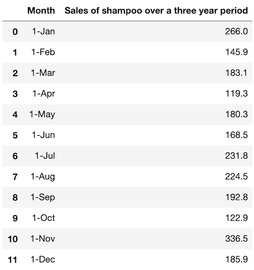
Once the dataset of three-year sales of shampoo in Kaggle [6] has been downloaded onto a local machine, the dataset csv file can be loaded into a Pandas DataFrame as follows:

df = pd.read_csv('./data/sales-of-shampoo-over-a-three-ye.csv')
df.head(12)

The column of sales in the DataFrame can be extracted as a time series dataset:

sales = df['Sales of shampoo over a three year period']
sales.plot(figsize=(16,5))

The following plot shows the sales of shampoo in three years (36 months):

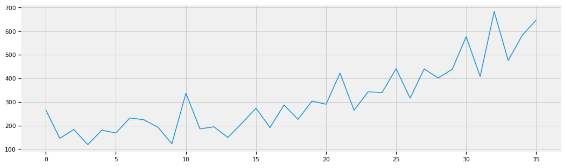
Figure 1: Sales of shampoo in three years (36 months).

4.2 Modeling

A good start to Bayesian modeling [3] is to think about how a given dataset might have been generated. Taking the sales of shampoo time series data in Figure 1 as an example, we can start by thinking:

• The dataset might have been generated by a linear function of time with random errors in sales since the dataset roughly forms a straight line from lower left corner to upper right corner.
• the random errors might follow a normal distribution with zero mean and an unknown standard deviation std.

We know that a linear function is determined by two parameters: slope beta and intercept alpha:

sales = beta x t + alpha + error

To estimate what the linear function of time might be, we can fit a linear regression machine learning model into the given dataset to find the slope and intercept:

import numpy as np
from sklearn.linear_model import LinearRegressionX1 = sales.index.values
Y1 = sales.values
X = X1.reshape(-1, 1)
Y = Y1.reshape(-1, 1)
reg = LinearRegression().fit(X, Y)reg.coef_, reg.intercept_

where reg.coef_ = 12.08 is the slope and reg.intercept_ = 101.22 is the intercept.

Y_reg = 12.08 * X1 + 101.22def plot_df(x, y, y_reg, title="", xlabel='Date', ylabel='Value', dpi=100):
    plt.figure(figsize=(16,5), dpi=dpi)
    plt.plot(x, y, color='tab:blue')
    plt.plot(x, y_reg, color='tab:red')
    plt.gca().set(title=title, xlabel=xlabel, ylabel=ylabel)
    plt.show()plot_df(x=X1, y=Y1, y_reg=Y_reg, title='Sales')

The above code plots the regression line in red over the sales curves in blue:

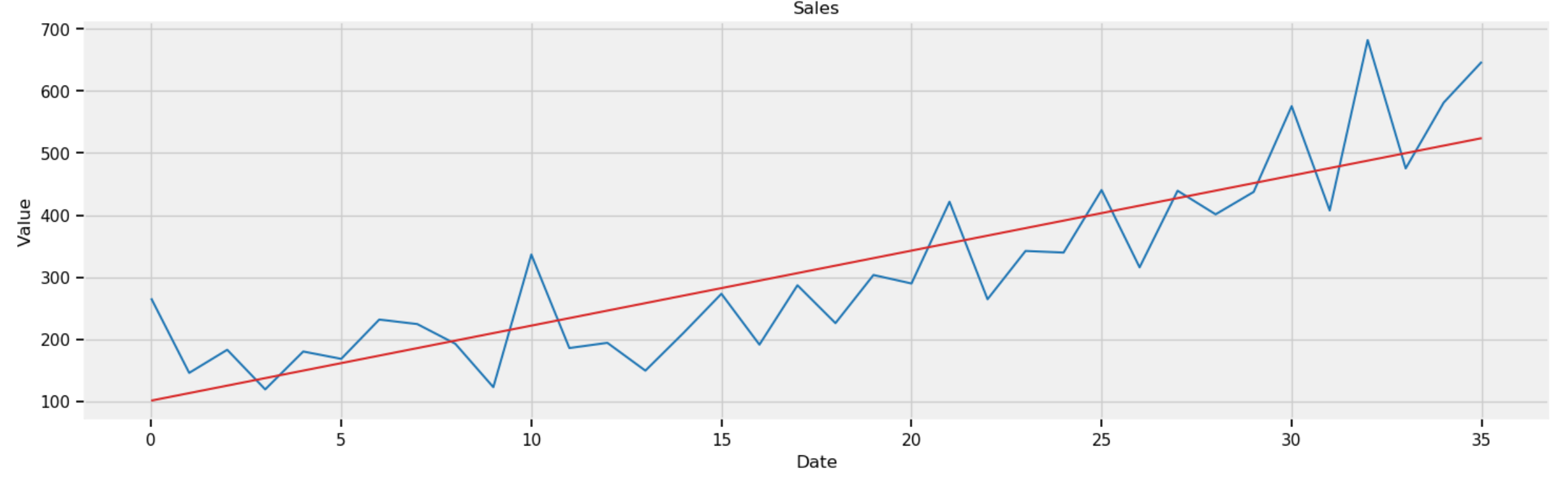
Figure 2: Sales of shampoo in three years (36 months) with regression line in red.

The slope and intercept of the regression line are just estimations based on limited data. To take care of uncertainty, we can represent them as normal random variables with the identified slope and intercept as mean values. This is achieved in PyMC [7] as below:

beta = pm.Normal("beta", mu=12, sd=10)
alpha = pm.Normal("alpha", mu=101, sd=10)

Similarly, to handle uncertainty, we can use PyMC to represent the standard deviation of errors as a uniform random variable in the range of [0, 100]:

std = pm.Uniform("std", 0, 100)

With the random variables of std, beta, and alpha, the regression line with uncertainty can be represented in PyMC [7]:

mean = pm.Deterministic("mean", alpha + beta * X)

With the regression line with uncertainty, the prior distribution of the sales of shampoo time series data can be programmed in PyMC:

obs = pm.Normal("obs", mu=mean, sd=std, observed=Y)

Using the above prior distribution as the start position in the parameters (i.e., alpha, beta, std) space, we can perform MCMC using the Metropolis–Hastings algorithm in PyMC:

import pymc3 as pmwith pm.Model() as model:
    std = pm.Uniform("std", 0, 100)
    
    beta = pm.Normal("beta", mu=12, sd=10)
    alpha = pm.Normal("alpha", mu=101, sd=10)
    
    mean = pm.Deterministic("mean", alpha + beta * X)
    
    obs = pm.Normal("obs", mu=mean, sd=std, observed=Y)
    
    trace = pm.sample(100000, step=pm.Metropolis())
    burned_trace = trace[20000:]

There are 100,000 accepted steps, called trace, in total. We ignore the first 20,000 accepted steps to avoid the burn-in period before convergence [3][4]. In other words, we only use the accepted steps after the burn-in period for Bayesian inference.

4.3 Posterior Analysis

The following code plots the traces of std, alpha, and beta after the burn-in period:

pm.plots.traceplot(burned_trace, varnames=["std", "beta", "alpha"])

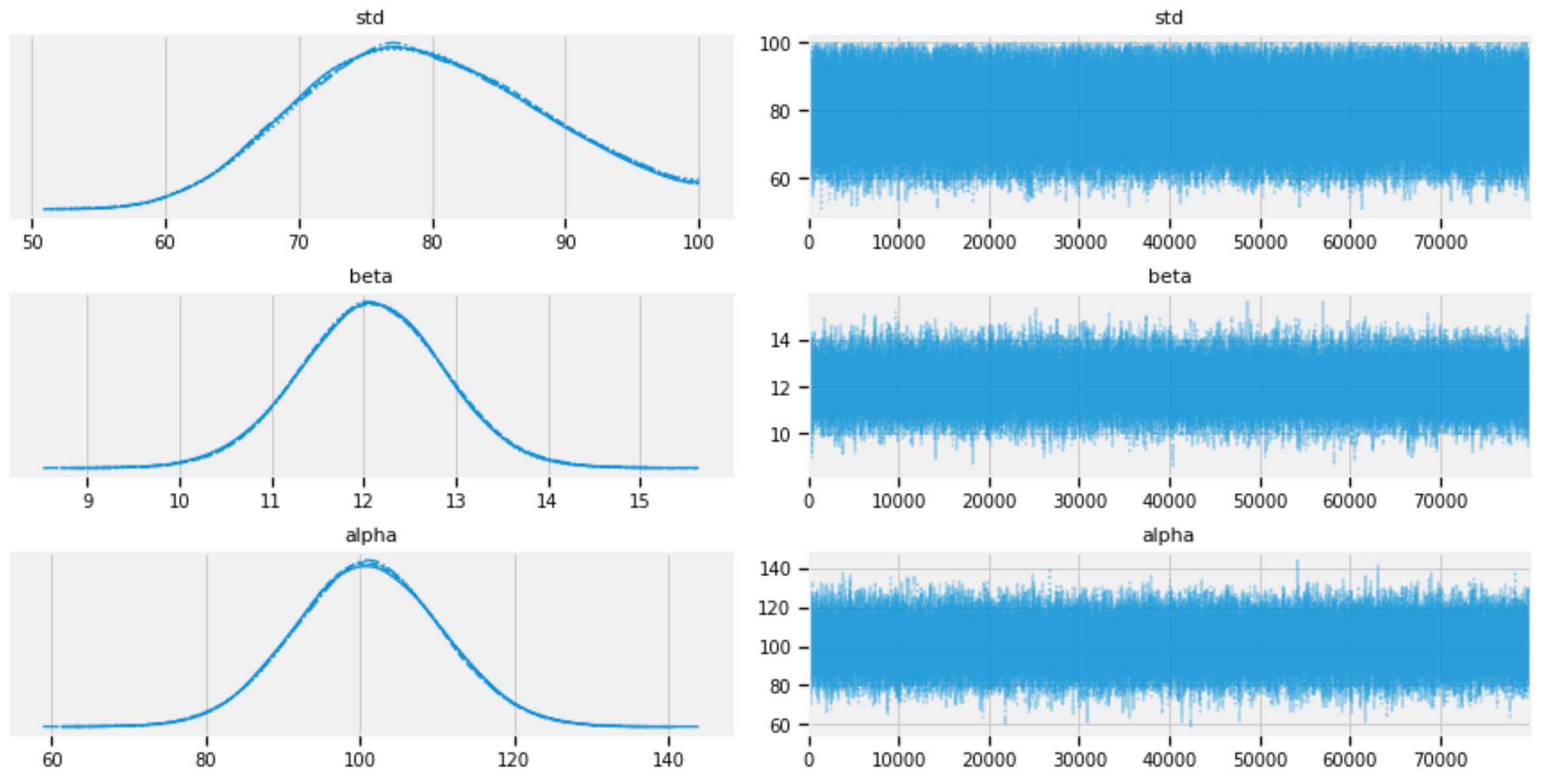
Figure 3: Traces of std, alpha, and beta.

The posterior distributions of std, alpha, and beta can be plotted as follows:

pm.plot_posterior(burned_trace, varnames=["std", "beta", "alpha"])

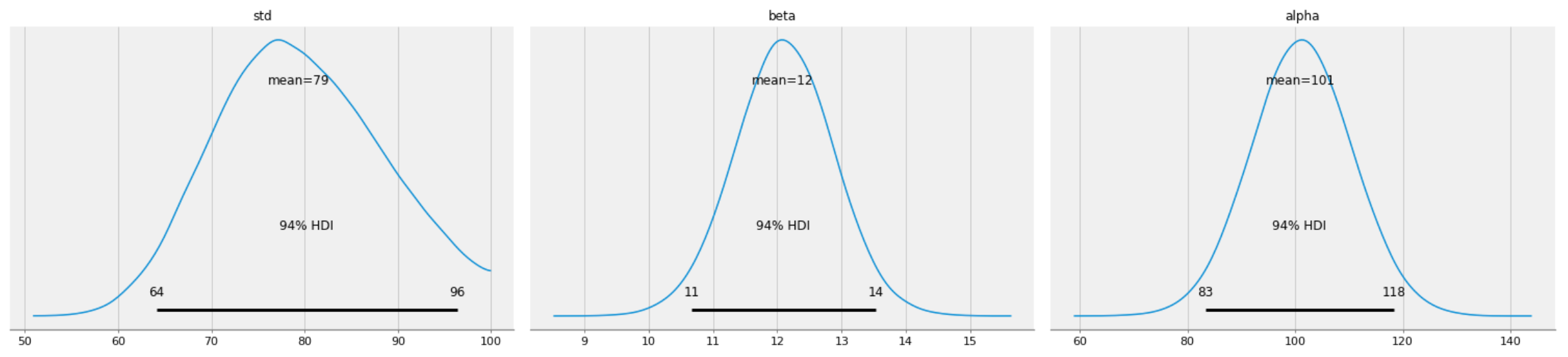
Figure 4: Posterior distributions of std, alpha, and beta.

The individual traces of std, alpha, and beta can be extracted for analysis:

std_trace = burned_trace['std']
beta_trace = burned_trace['beta']
alpha_trace = burned_trace['alpha']

We can zoom into the details of the trace of std with any specified number of steps (e.g., 1,000):

pd.Series(std_trace[:1000]).plot()

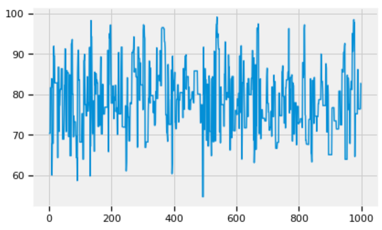
Figure 5: Zoom into the trace of std.

Similarly we can zoom into the details of the traces of alpha and beta respectively:

pd.Series(beta_trace[:1000]).plot()

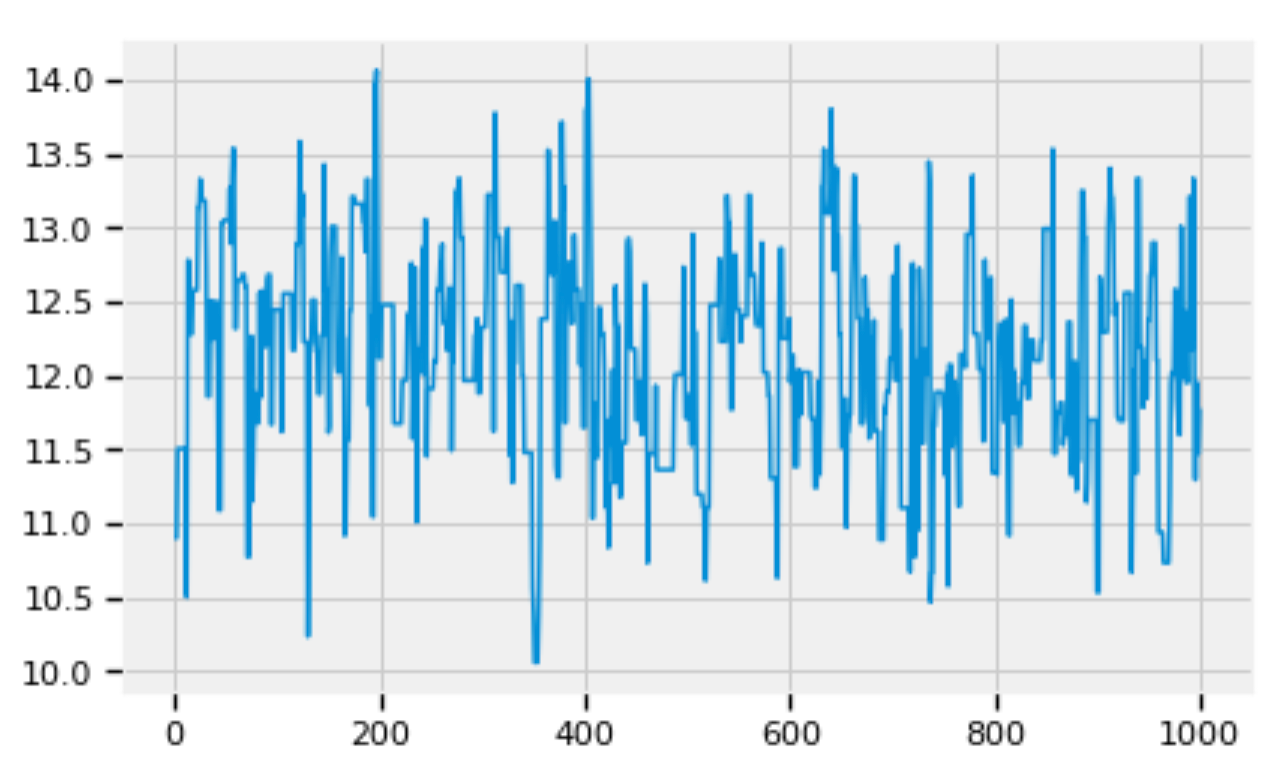
Figure 6: Zoom into the trace of beta.

pd.Series(alpha_trace[:1000]).plot()

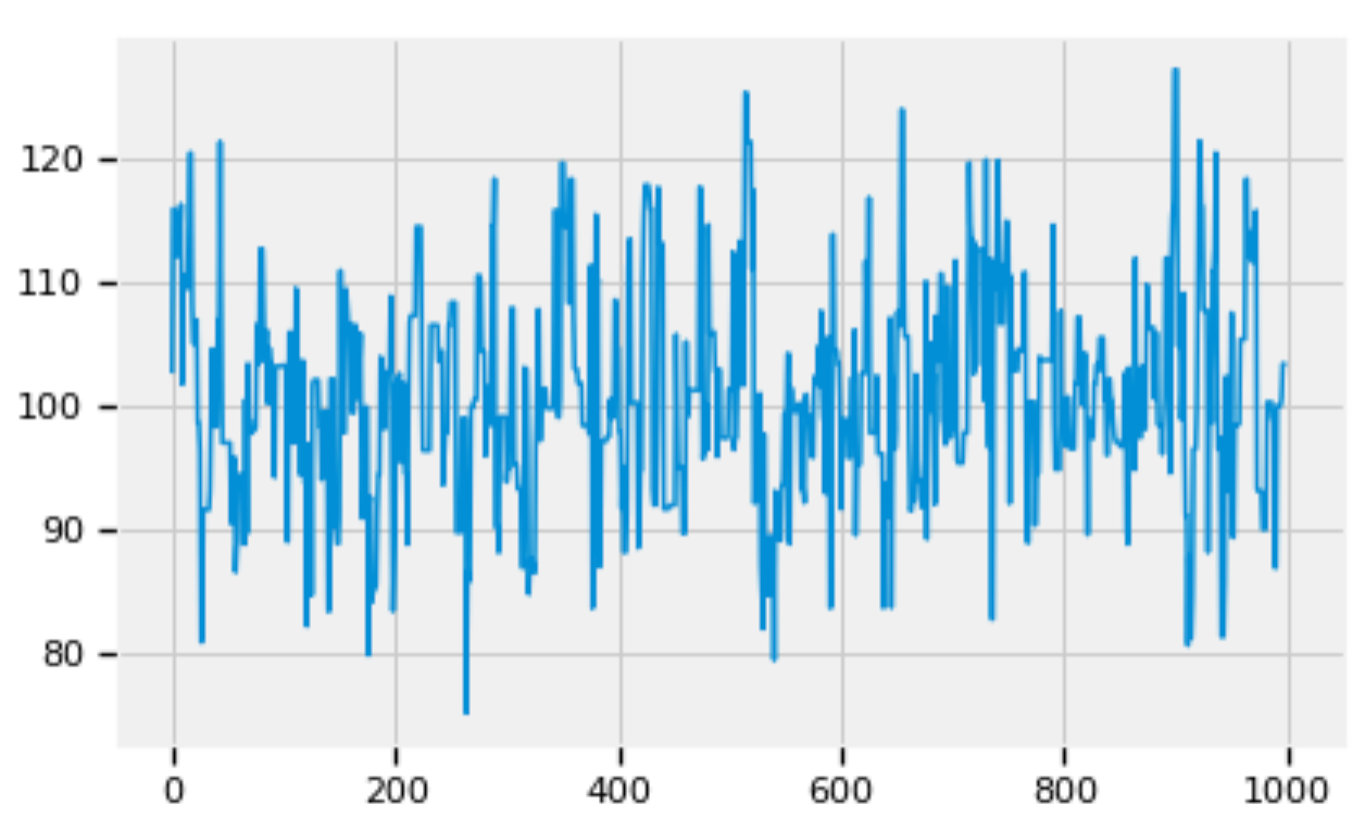
Figure 7: Zoom into the trace of alpha.

Figures 5, 6, and 7 show that the posterior distributions of std, alpha, and beta have well mixed frequencies and thus low autocorrelations, which indicate MCMC convergence [3].

4.4 Forecasting

The mean values of the posterior distributions of std, alpha, and beta can be calculated:

std_mean = std_trace.mean()
beta_mean = beta_trace.mean()
alpha_mean = alpha_trace.mean()

• std_mean = 79.41
• beta_mean = 12.09
• alpha_mean = 101.03

The forecasting of the sales of shampoo can be modeled as follows:

Sale(t) = beta_mean x t + alpha_mean + error

where error follows normal distribution with mean of 0 and standard deviation of std_mean.

Using the model above, given any number of time steps (e.g., 72), we can generate a time series of sales:

length = 72
x1 = np.arange(length)
mean_trace = alpha_mean + beta_mean * x1
normal_dist = pm.Normal.dist(0, sd=std_mean)
errors = normal_dist.random(size=length)
Y_gen = mean_trace + errors
Y_reg1 = mean_trace

Given 36 months of data, the code below plots the forecasting of sales in the next 36 months (from Month 37 to Moth 72).

plot_df(x=x1, y=Y_gen, y_reg=Y_reg1, title='Sales')

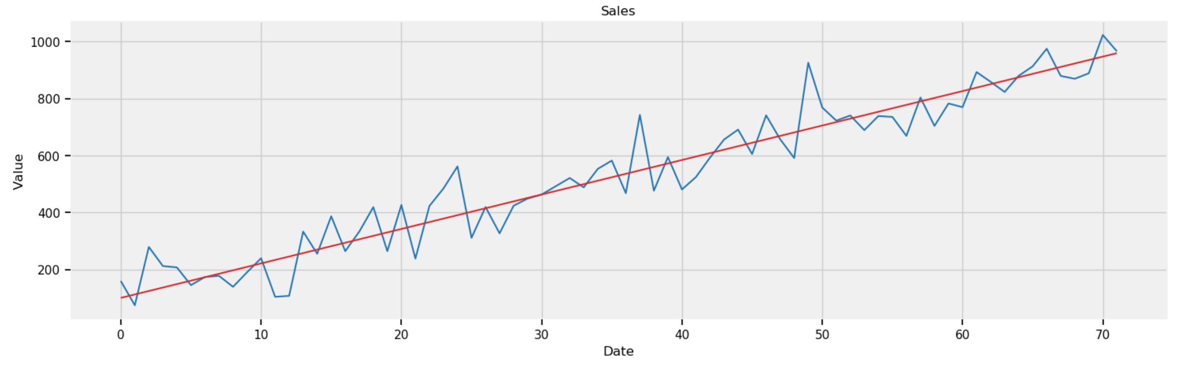Figure 8: Forecasting sales in next 36 months (from Month 37 to Month 72).

 

5. Summary

In this article, I used the small Sales of Shampoo [6] time series dataset from Kaggle [6] to how to use PyMC [3][7] as a Python probabilistic programming language to implement Bayesian analysis and inference for time series forecasting.

The other alternative of probabilistic programming language is the Tensorflow probability [8]. I chose PyMC in this article for two reasons. One is that PyMC is easier to understand compared with Tensorflow probability. The other reason is that Tensorflow probability is in the process of migrating from Tensorflow 1.x to Tensorflow 2.x, and the documentation of Tensorflow probability for Tensorflow 2.x is lacking.

References

1. Common Time Series Data Analysis Methods and Forecasting Models in Python
2. R.H. Shumway and D.S. Stoffer, Time Series Analysis and Its Applications with R Examples, 4th Edition, Springer, 2017
3. C. Davidson-Pilon, Bayesian Methods for Hackers, Probabilistic Programming and Bayesian Inference, Addison-Wesley, 2016
4. J.K. Kruschke, Doing Bayesian Data Analysis, A Tutorial with R, JAGS, and Stan, Academic Press, 2015
5. A.B. Downey, Think Bayes, O’Reilly, 2013
6. Sales of Shampoo Over a Three Year Period
7. PyMC3
8. Tensorflow Probability
9. Jupyter notebook in Github