In commercial settings, Machine Learning is far more prevalent than Bayes Nets. But do Bayes Nets have capabilities beyond what machine learning has to offer? When it comes to scenarios that involve probability and causation, the answer is yes.

The difference between results from machine learning models and a Bayes Net is that the latter can tell you how likely it is to see a specific pattern of data if a particular hypothesis is true.

A Bayes Net is a probabilistic generative model. A generative means you already know something and start with a hypothesis). A machine learning model can manipulate data to find relationships, patterns and provide the data-based means to make predictions without probability.

Commercial applications of “AI,” which is a loosely defined term, use algorithms with carefully chosen but usually vast datasets to find patterns in the data for classification and prediction. Most Machine Learning algorithms use the GLM, the Generalized Linear Model, also known as regression. A regression finds a linear (straight line) to run through a series of dots in an XY plane in the simplest form. That minimizes the sum of the (squared) vertical distances between the regression line and the dots, as in the picture below:

The breadth of GLM models is broad, covering many different statistical models: ANOVA,  ANCOVA,  MANOVA, MANCOVA, ordinary linear regression, t-test, and F-test. The underlying probability functions include Poisson, Laplace, Gamma, and dozens of others. But still, the model itself has no intelligence whatsoever. It’s just math.

One controversial aspect of AI is the process of labeling. A candidate dataset is prepared and divided between “test” data and “proof” data. The developer labels the test dataset (“horse,” “cow,” Ducati,” “horse,” “ET”), contracts a data labeling service, or purchases labeled data from a third party (an excellent review of the issues of labeling is here: The Ultimate Guide to Data Labeling for Machine Learning).

As you can see from the linked content, 80% of the work does not involve AI or data science expertise. It is just wrangling the data. Once the portion of the set is labeled, the ML algorithm runs against it to find what other features are predictive of a horse (OK, I already know this is a horse, what other features are related). If the “ground truth” (satisfaction – it performs well), the model is turned against the unlabeled data to see if the predictors discovered in the training phase are acceptable.

They usually aren’t. It’s an iterative process. The output of a machine learning run can be something like, “If a1 is false and a2 is true and a3 > 3 <11 … it’s a horse).” This is very useful in finding pictures of horses if that is your objective, but it’s also useful for a multitude of other things.

One prevalent way of doing ML is not labeling the data at all, and letting the ML model find commonality in the data to create clusters. A growing and beneficial application assists in creating and maintaining semantic metadata (see my article Metadata Shmedadata). This is a rapidly improving approach to harmonizing data from many sources and the design of data catalogs in a partially unsupervised manner. All of these disciplines are “bottom-up” processes, using algorithms to process vast sets of data. The drawback is that data rarely speaks for itself – or by itself.

Things that become questionable are problems in optimization scenarios based not on the best fit, but on a range of solutions that fit the criteria. A Bayesian approach would be a Hierarchical Constraint Resolution Model. An excellent introduction to Hierarchical Constraint modeling is Solving Hierarchical Constraints over Finite Domains with Local Search. ML would use a brute force method that could take quite a bit of time, not acceptable to near real-time applications, such as edge analysis of sensor data.

Uncertainty and causation – two machine learning weaknesses

But two things are missing in machine learning output: uncertainty and causation.

In general, ML techniques are referred to as bottom-up. There are also robust and mature techniques to create useful “top-down” methods-these approaches provide measures of uncertainty with probable outcomes and a shot at causation. Top-down approaches, like Bayesian models, address critical issues of uncertainty and causation. A Bayesian model produces probabilities of outcomes and, in most cases, a pretty clear understanding of causation, too, something that is missing in ML, until the operator offers an interpretation of the results. Bayesian statistics use probabilities to attack statistical problems and provide for people to update their conclusions as new data enters the model. But using probabilistic reasoning is still a problem.

Probability can be very counter-intuitive. If you flip a coin, the probability of it turning up heads is 50%. But once joint probability or conditional probability (Bayesian) gets into the mix, our decision-making rarely involves probability instead of heuristics or deterministic models (think about the annual budget). When asking for your investigation results, does it matter if you say 85% probability of 95%? Our management gestalt doesn’t work that way.

As a demonstration: is a problem where three students whose chances of solving a problem are 1/2, 1/3, and 1/4, respectively. What is the probability that will solve the problem?

Probability can be confusing. While there is ostensibly some arithmetic involved, probability is not precisely math. While it applies math to be concise, sometimes it gets in the way., like this example. The math is incidental. The important thing to solving the problem is thinking through the steps. This presents a problem to many data scientists, and is in opposition to companies’ current craze to be “data-driven.”

Judea Pearl, the “inventor” of Bayesian Belief Networks, previously quoted in a recent diginomica  article, pointed out (his perception) of the difference between Bayes Nets and ML:

AI is currently split. First, some are intoxicated by the success of machine learning and deep learning and neural nets. They don’t understand what I’m talking about. They want to continue to fit curves. But when you talk to people who have done any AI work outside statistical learning, they get it immediately. I have read several papers written in the past two months about the limitations of machine learning.

Pearl did win the Turing Award, so his opinion is worth considering. Realistically, to refer to everything other than Bayes Nets as “curve fitting” is an exaggeration (but). It is possible he was a little sarcastic. Pearl later modified his statement to provide that many useful results can and have been produced by the application of ML. His point is that Bayesian inference, in particular, can add crucial clarity to complex decisions. Many AI/ML algorithms are very productive and can offer significant value, provided organizations are willing (and able) to incorporate them into decision-making activities.

Bayesian networks – a simple example

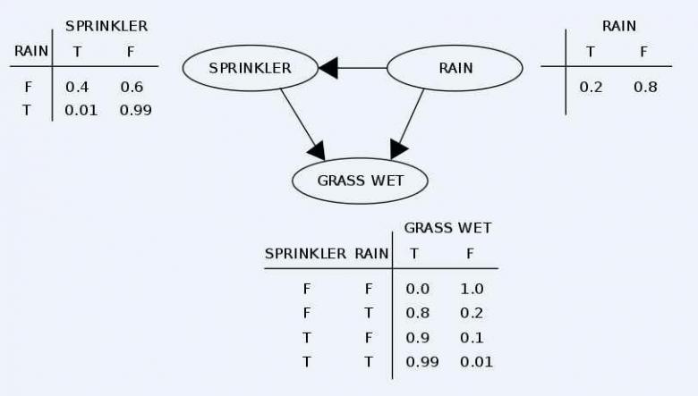
Bayesian Networks can be described as directed acyclic graphs (DAGs). Think of a graph as a set of tinker toys. The connectors represent the nodes, and the sticks represent the edges. The tables in the graphic below represent the conditional probabilities, what you know. Nodes are observable quantities, unknown parameters, or hypotheses and latent variables (that are not directly observed but are instead inferred). Edges are conditional dependencies:

Two events can cause the grass to be wet: an active sprinkler or rain. The rain directly affects the sprinkler’s use (namely that when it rains, the sprinkler is usually not active). This situation can be modeled with a Bayesian network. Each variable has two possible values, T (for true) and F (for false).

The joint probability function is:

where G = “Grass wet (true/false)”, S = “Sprinkler turned on (true/false)”, and R = “Raining (true/false)”.

Pr(G,S,R) = Pr(G|S,R) Pr(S|R) Pr(R)

This model can answer questions about the presence of a cause given the presence of an effect (so-called inverse probability) like “What is the probability that it is raining, given the grass is wet?”

This is a simple example. In operation, a Bayes Net can be very complicated.

My take

In part II, we’ll dig into Bayesian Inference and some examples.  Suppose Bayesian Nets are superior to machine leering in understanding uncertainty and causation, and more economical in terms of data needed and the power consumption of computers? Why have they not been as widely used? The answer is: our business and government cultures are not accustomed to responses involving probability.

It’s the difference between “This merger will not go well,” as opposed to “This merger has at most a 76% probability in ending satisfactorily.” An executive’s response to the last answer is likely to be, “What does that mean? Is that good or bad?” And that’s a good question. How does one judge an answer with a probability? On the other hand, causation is rarely part of a machine learning application, beyond the engineer’s interpretation of the results. Adding causative explanations to probability can go a long way to interpreting them.