
Probabilistic Programming and Bayesian Inference for Time Series Analysis and Forecasting in Python
July 28, 2020


Undoubtedly, randomized experimentation (assuming it is conducted properly) is the most straightforward way to establish causality (refer to my previous article on a collection of A/B testing learning resources!). However, practically speaking, there are cases when experimentation is not a viable option:
Cases above are frequently referred to as observational studies, where the independent variable is not under the researchers’ control. Observational studies reveal a fundamental problem in measuring causal effect — that is, whatever change we observe between treatment and non-treatment groups is counterfactual, meaning we don’t know what would have happened to people in the treatment group if they had not received the treatment.
Drawing theories from well known statistical books, research papers, and course lecture notes, this article presents 5 different approaches to making counterfactual inferences in the presence of non-experimental data. Simple code examples and applications in the tech industry are also included so that you can see how theory is put into practice.
Scenario: Imagine a hypothetical scenario, where you release a new feature to your whole user base, and want to measure the impact of that feature on users’ overall engagement level (e.g. a composite index to measure engagement). You collect data from your whole user base, and want to regress engagement index on # of new feature clicks. Is this a sound approach?
Theory: Most likely the answer is NO. In the case above, we try to measure the impact of new feature usage on users’ overall engagement levels (left causal graph in Plot I below).
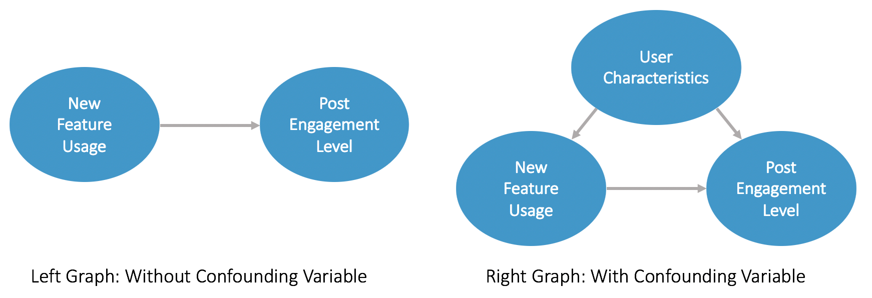
However, there are likely confounding variables that are omitted from the model and have an impact on both the independent variable and the dependent variable. Such confounding variables may include users’ characteristics (e.g. age, region, industry, etc.). Very likely, those user characteristics determine how frequently users will use the new feature, and what their post-release engagement levels are (see the right causal graph in Plot 1 above). Those confounding variables need to be controlled for in the model.
Example Code: Assuming that you have 10k MAU…
## Parameter setup
total_num_user = 10000
pre_engagement_level = rnorm(total_num_user)
new_feature_usage = .6 * pre_engagement_level + rnorm(total_num_user)
post_engagement_level = .4 * pre_engagement_level + .5 * new_feature_usage + rnorm(total_num_user)## Model without the confounder
summary(lm(post_engagement_level~new_feature_usage))## Model with the confounder
summary(lm(post_engagement_level~new_feature_usage+pre_engagement_level))
And the first regression incurs an upward bias on the coefficient estimate, due to the positive impact of the confounder on both the independent and the dependent variable.
When this approach won’t work: Now you may wonder, will controlling for confounders always work? NO. It works only if the following assumptions are met [1]:
We will move on and talk about other methods to use when these assumptions don’t hold true.
Theory: When the treatment and non-treatment groups are not comparable, that is, when the distributions or the ranges of the confounding covariates vary across the control and treatment groups, the coefficient estimates are biased [1]. Matching techniques ensure balanced distribution by identifying pairs of data points in treatment and non-treatment groups that are close to each other, with the confounding covariates defining the distance between the pair. Those techniques output a smaller dataset where each treatment observation matches with one (or more) non-treatment observations that are the closest to it.
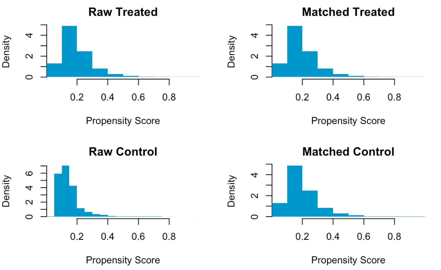
The matching process can be expensive for models with numerous pre-treatment variables. Propensity Score Matching (PSM) simplifies the problem by calculating a single score for each of the observations, which can then be used to identify the matched pair (see example on the left, generated using example code below).
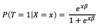
Propensity scores are often estimated using standard models such as logistic regression, with the treatment variable being the dependent variable (T) and confounding covariates (X) being the independent variables. It thus estimates the probability of an individual receiving the treatment, conditioned by confounding covariates.
Industry Application: As an alternative to A/B testing, this method has been applied by researchers at tech companies as well. For instance, LinkedIn published a paper in 2016 to share the use of quasi-experimental methods in its mobile app adoption analysis. The complete revamp of the mobile app UI along with the infrastructure challenges made it infeasible for A/B testing. With the help of historical release data, they proved how Propensity Score techniques reduce adoption bias and can be used to measure the impact of major product releases [2].
Example Code: R’s Matchit Package provides a variety of ways to select the matched pairs using different distance definitions, matching techniques, etc., and we will illustrate it in the following example. In the code example below, we use a sample of the 2015 BRFSS survey data accessible through the University of Virginia library. This sample has 5000 records and 7 variables, and we are interested in understanding the effect of smoking on chronic obstructive pulmonary disease (CODP), after controlling for race, age, gender, weight and average drinking habits covariates.
## Read in data and identify matched pairs
library(MatchIt)
sample = read.csv("http://static.lib.virginia.edu/statlab/materials/data/brfss_2015_sample.csv")
match_result = matchit(SMOKE ~ RACE + AGE + SEX + WTLBS + AVEDRNK2,
                       data = sample,
                       method = "nearest",
                       distancce = "logit")
par(family = "sans")
plot(match_result,  type = "hist", col = "#0099cc",lty="blank")
sample_match = match.data(match_result)## Models with imbalanced and balanced data distribution
sample$SMOKE = factor(sample$SMOKE, labels = c("No", "Yes"))
sample_match$SMOKE = factor(sample_match$SMOKE, labels = c("No", "Yes"))
mod_matching1 = glm(COPD ~ SMOKE + AGE + RACE + SEX + WTLBS + AVEDRNK2, data = sample, family = "binomial")
mod_matching2 = glm(COPD ~ SMOKE + AGE + RACE + SEX + WTLBS + AVEDRNK2, data = sample_match, family = "binomial")
summary(mod_matching1)
summary(mod_matching2)
Theory: When assumption b) is not met, that is, when there are confounding variables that can not be observed, the use of Instrumental Variable (IV) can reduce the omitted variable bias. A variable Z qualifies as an instrumental variable if : 1) Z is correlated with X; 2) Z is not correlated with any covariants(including error terms) that have an influence on Y [3]. Those conditions imply that Z influences Y only through its effect on X. Thus, changes in Y caused by Z are not confounded and can be used to estimate the treatment effect.
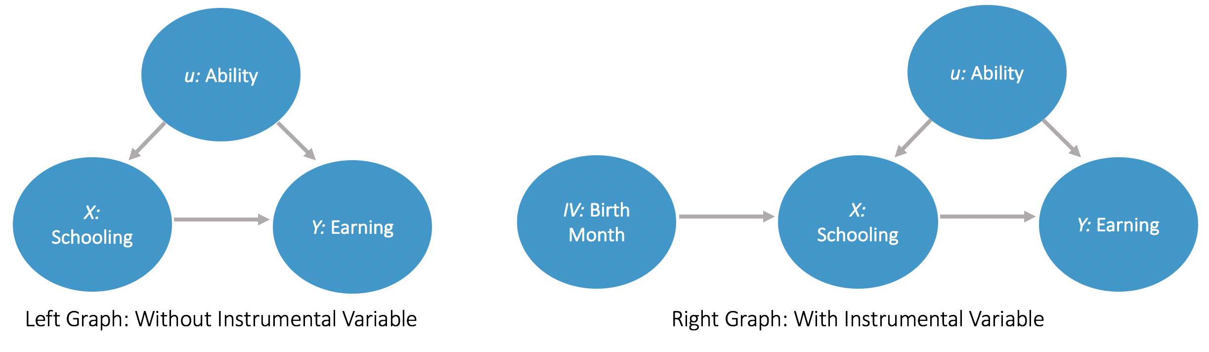
For example, to study the impact of schooling (e.g. years of education) on earning, “ability” is an important though hard-to-measure variable, which has an impact on both how well students do in school, as well as their earning post-school. One Instrumental Variable that researchers have studied is month of birth, which determines the school entrance year and thus years of education, but at the same time has no impact on earning (illustrated in Plot 3).
In practice, IV is often estimated using two-stage least squares. During the first stage, IV is used to regress on X to measure the covariance between X & IV. During the second stage, predicted X from the first stage, along with other covariates are used to regress Y, thus focusing on the changes in Y caused by the IV.
The biggest challenge of this method is that instrumental variables are hard to find. In general, IVs are more widely used in econometric & social science studies. Thus, industry applications & code examples are omitted here.
Theory: When there are no good candidates of IVs, we need an alternative way to account for the unobserved covariates. Difference-in-differences (DiD) method works by comparing the control & treatment groups’ post-treatment differences to the pre-treatment differences, assuming the two groups’ dependent variables would have followed a similar trend if there was no intervention. Unlike Matching/PSM that try to identify pairs of data points that are similar to each other, the DiD estimator takes into account any initial heterogeneity between the two groups.
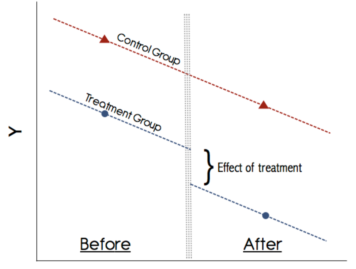
The key assumption for the DiD method is that the dependent variable in control & treatment groups follows the same trends (the parallel world assumption). This doesn’t mean they need to have the same average value or that there is no trend at all during the pre-treatment period [4]. See an example plot on the left where control & test groups have similar trends during the pre-treatment period. If the assumption holds true, the post-treatment differences in the treatment group can be decomposed into the difference that is similarly observed in the control group, and the difference caused by treatment itself. DID is usually implemented as an interaction term between time and treatment group dummy variables in a regression model.

And there are a few different ways to validate the parallel world assumption. The simplest way is to do a visual inspection. Alternatively, you can have the treatment variable interact with the time dummy variables to see if the difference in differences between the two groups is insignificant during the pre-treatment period [5].
Industry Application: Similar to Propensity Score Matching, this method has been favored by tech companies who want to study user behaviors in non-experimental settings. For instance, Facebook in their 2016 paper applies the DiD approach to study how contributors’ engagement levels change before and after posting to Facebook. They found that after posting content, people “are more intrinsically motivated to visit the site more often…”[6]. This is another good example where the behavior of posting or not is out of the researchers’ control, and can only be analyzed through causal inference techniques.
Example Code: Here we are looking at how to use DiD to estimate the impact of the 1993 EITC (Earned Income Tax Credit) on employment rate of women with at least one child. Credit to [7] & [8] for the original analysis and the below code is just a simplified version to demo how DiD works!
## Read in data and create dummy variables
library(dplyr)
library(ggplot2)
data_file = '../did.dat'
if (!file.exists(data_file)) {
    download.file(url = 'https://drive.google.com/uc?authuser=0&id=0B0iAUHM7ljQ1cUZvRWxjUmpfVXM&export=download', destfile = data_file)}
df = haven::read_dta(data_file)
df = df %>%
    mutate(time_dummy = ifelse(year >= 1994, 1, 0),
           if_treatment = ifelse(children >= 1, 1, 0))## Visualize the trend to validate the parallel world assumption
ggplot(df, aes(year, work, color = as.factor(if_treatment))) +
    stat_summary(geom = 'line') +
    geom_vline(xintercept = 1994)## Two ways to estimate the DiD effect: shift in means & regression
var1 = mean( (df %>% filter(time_dummy==0 & if_treatment==0 ))$work)
var2 = mean( (df %>% filter(time_dummy==0 & if_treatment==1 ))$work)
var3 = mean( (df %>% filter(time_dummy==1 & if_treatment==0 ))$work)
var4 = mean( (df %>% filter(time_dummy==1 & if_treatment==1 ))$work)
(var4 - var3) - (var2 - var1)mod_did1 = lm(work~time_dummy*if_treatment, data = df)
summary(mod_did1)
Despite DiD being a popular causal inference approach, it has some limitations:
A recent line of research based on state-space models generalizes DiD for more flexible use cases by utilizing fully Bayesian time-series estimate for the effect, and model averaging for the best synthetic control [9]. The Google publication and the corresponding R Package “CausalImpact” show both the theory behind and implementation of such state-space models, and are recommended for further reading.
References:
[1] Andrew Gelman and Jennifer Hill. “Data Analysis Using Regression and Multilevel/Hierarchical Models” (2007)
[2] Evaluating Mobile Apps with A/B and Quasi A/B Tests. https://dl.acm.org/citation.cfm?id=2939703
[3] Pearl, J. (2000). Causality: Models, reasoning and inference. New York: Cambridge University Press.
[4] Lecture Notes: Difference in Difference, Empirical Method http://finance.wharton.upenn.edu/~mrrobert/resources/Teaching/CorpFinPhD/Dif-In-Dif-Slides.pdf
[6] Changes in Engagement Before and After Posting to Facebook https://research.fb.com/publications/changes-in-engagement-before-and-after-posting-to-facebook/
[7] https://thetarzan.wordpress.com/2011/06/20/differences-in-differences-estimation-in-r-and-stata/
[9] Inferring causal impact using Bayesian structural time-series models https://research.google/pubs/pub41854/
Source https://towardsdatascience.com/causal-inference-thats-not-a-b-testing-theory-practical-guide-f3c824ac9ed2
Probabilistic Programming and Bayesian Inference for Time Series Analysis and Forecasting in Python
July 28, 2020

Efficient Intervention Design for Causal Discovery with Latents
June 3, 2020

May 20, 2020

A Guided Tour of Artificial Intelligence Research
May 14, 2020
AI World Society - Powered by BGF